 EPOCH IDLE
From One Line to a Transformer: Machine Learning in Four Eras
Every modern language model still runs the same core loop Frank Rosenblatt wired into hardware in 1958: guess, measure the error, nudge the dials, repeat.
If you strip away the cluster engineering and the billion-dollar budgets, training a neural network comes down to four things:
- Parameters (
θ): a list of adjustable numbers inside the model. - A forward pass: plugging input data
xinto those numbers to make a prediction. - A loss function (
L): a single score measuring how wrong the prediction was. - An update rule: nudging the parameters in the direction that shrinks the loss.
That loop has not changed in seventy years. What changed is the shape of the function between input and output. And in the history of machine learning, researchers only changed that function when the old one hit a mathematical wall it provably could not cross.
Era 1: Two Dials and a Straight Line (1958)
Suppose you have ten noisy data points on a graph and you want a formula that predicts height y from position x. The simplest possible model is a straight line:
When the model starts cold, w and b are wrong. To measure how wrong, we take the vertical distance between each point and the line, square it so negative and positive errors don't cancel out (and so big misses get punished hard), and average them. That is Mean Squared Error (MSE).
We don't guess new values for w and b at random. We take the derivative of the error with respect to each dial (the gradient, ∇L), which points uphill toward worse error, and step the opposite way, scaled by a step size called the learning rate (η).
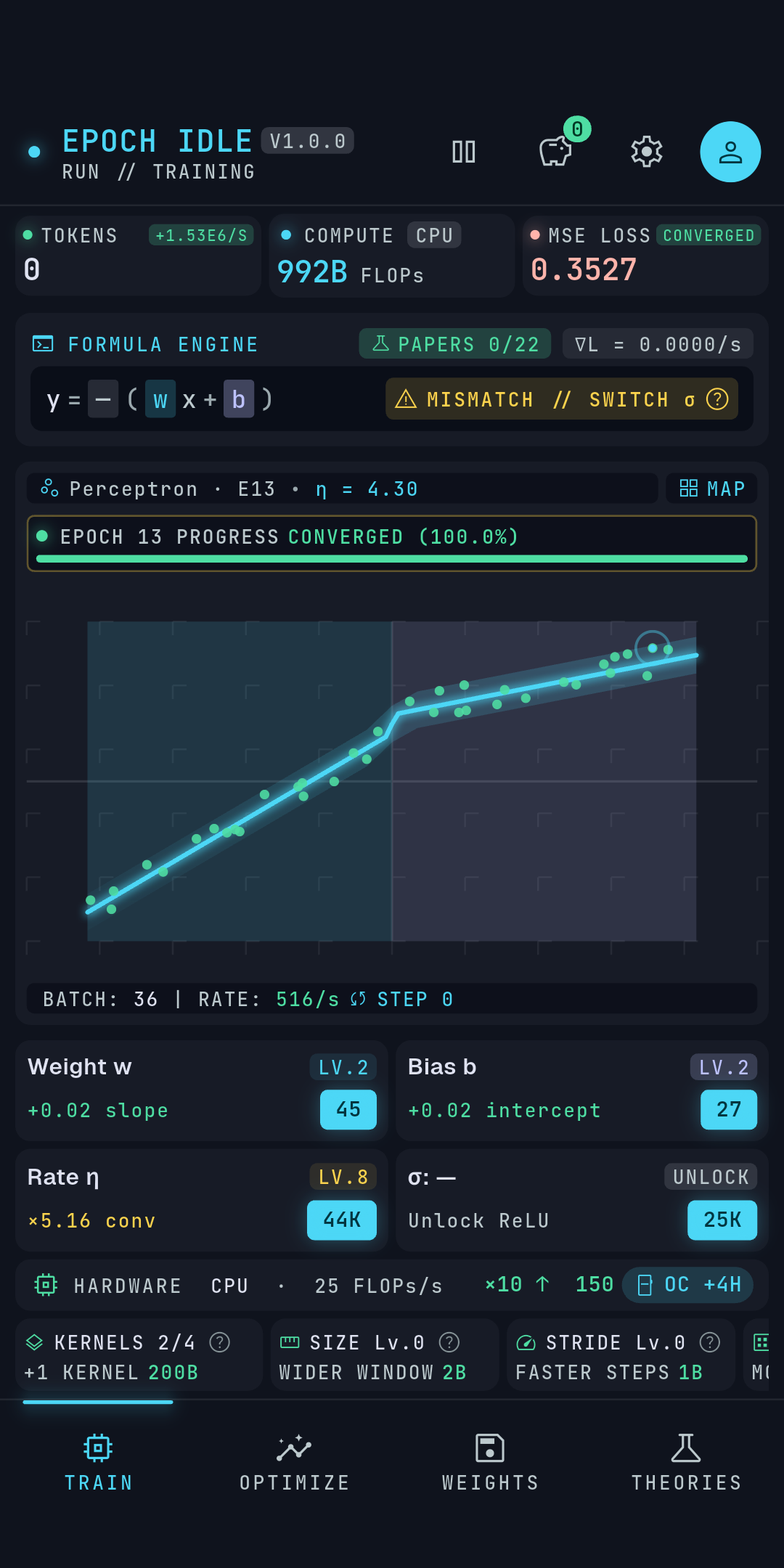
Try it yourself below. Drag w and b, or click STEP −∇L to let gradient descent walk them onto the points:
Notice that the loss never hits zero. The data points have random measurement noise (σ) baked into them. Once your line sits right on the true underlying slope, the normalized loss settles near 1.0. That flat bottom is convergence. Any further training is wasted electricity.
Era 2: The Non-Linear Wall (1969 → 2012)
In the widget above, click DATASET E3 (HINGE) and keep the activation on σ: LINEAR. Now click STEP −∇L a few times.
The line tilts, shifts, and then gets stuck around L ≈ 2.40. The status badge flips to CEILING // σ REQ. The left half of the dataset is flat at zero; the right half climbs steeply. No single straight line can lie flat on the left and angle up on the right at the same time.
Worse, stacking more linear layers doesn't help. If layer one computes y = w₁x + b₁ and layer two computes z = w₂y + b₂, basic algebra collapses the whole stack back into one line: z = (w₂w₁)x + (w₂b₁ + b₂). A thousand-layer linear network has the exact same expressive power as a one-layer linear network.
To bend the curve, you have to wrap the linear sum in a non-linear activation function (σ). Click σ: ReLU in the sandbox above and step again. ReLU (max(0, z)) clamps negative outputs to zero, creating a hinge. In two steps, the curve snaps onto the data and converges.
From Epoch 3 onward, datasets take shapes from one activation family: sharp hinges (ReLU), S-curves (Sigmoid), or smooth probabilistic hinges (GELU). If you have the wrong σ selected, the formula engine warns CEILING // σ REQ and tells you the exact analytic floor you're stuck on.
Era 3: Local Experts and Convolutions (1998 → 2012)
One hinge is enough for a single bend. What if the dataset has three distinct regions with different slopes - say, rising on the left, dropping in the middle, and rising again on the right?
A single global formula can't fit piecewise structure. Instead of stretching one equation across the whole domain, convolutional networks (CNNs) tile the input with small local windows called kernels. Each kernel only looks at a narrow slice of x (its receptive field), while sharing update gradients across the stack.
Here is where every beginner hits the second great trap of machine learning: if 4 kernels fit well, won't 8 kernels fit twice as well?
No. Every kernel has parameters to estimate from the handful of data points that fall inside its window. When you pack too many parameters onto too few samples, the kernels start fitting the random vertical noise of individual points instead of the true trend. Training loss looks great, but error on new, unseen points explodes. That gap is overfitting, and only more data (or data augmentation) cures it.
Era 4: Multi-Head Attention & Sparse Transformers (2017 → Today)
Convolutions dominated computer vision because adjacent pixels belong together. Language breaks that assumption. In the sentence "The server that we migrated three weeks ago after the outage finally crashed," the verb crashed links back to server eleven words earlier, skipping everything in between.
Fixed local windows cannot route across arbitrary distances without stacking dozens of blurry layers. In 2017, Vaswani et al. published Attention Is All You Need and threw out local windows entirely. Multi-Head Attention lets every position compare itself against every other position directly, building an N × N routing grid based on content rather than distance.
That global reach comes with a steep bill: comparing every token against every other token costs N² compute as the context window (N) grows. And once a single dense Transformer gets large enough, running every parameter on every token becomes wasteful - which is why frontier models pivoted again to Sparse Mixture-of-Experts (MoE), where a router wakes up only a few specialized sub-networks per token.
Train from a scalar perceptron to a Sparse Transformer
Every era in this article is a playable stage in Epoch Idle. Watch the live loss curve bend, debug overfitting, climb the SGD → Adam optimizer tree, and publish all 32 milestone papers.